Searching

 

 

 

 

 

 

 

A fundamental operation of a computer is to store huge information (called information storage) and retrieve information as quick as possible (called information retrieval). We have studied that sorting plays an important role in the task of information storage, whereas searching plays a pivotal role in the task of information retrieval.

Like sorting, searching is also an interesting problem in its own right. Searching methods are governed with how data are stored in computer, either in internal memory or in external memory. Searching methods are also decided by the data structure used to store information. In addition to this, searching methods are also decided by search over a small set of data to a large set of data. Searching, in general is the most time consuming task in many applications and the application of a good searching method eventually leads to a substantial increase in performance.

    In fact, several searching techniques have been proposed and it is not possible to cover all of them in a book of limited volume like this. A classification of all searching methods is shown in Figure 13.1.   It can be noted that all searching methods can be broadly classified into two categories: internal and external searching. A searching method is termed as internal search that is, searching involved with data, which are entirely stored in the internal memory of a computer. All internal searching methods again are either of two types: with key comparisons and without any comparisons. There are two sub classes in the class of searching with key comparisons: linear search when data are stored with linear data structures like array, table, linked list etc. and non-linear search where data are stored with non-linear data structures like tree, graphs, set etc. In addition to these, external searching methods are also known which deal with a large volume of data and stored in external storage device like magnetic tapes, disks, drums etc.

In this chapter we shall study various internal searching methods and analyze their performances. Before going to discuss all searching methods, we shall familiarize ourselves with the terminologies frequently will be referred in our discussions.

 

 

BASIC TERMINOLOGIES

Throughout the discussion of this chapter, some terms related to searching will be referred. These terms are defined in this section.

 

Key. This is the element to be searched. In fact, key is(are) a special field(s) in a record with which the record can be uniquely identified.

 

Item. Same as the key. It is an element under search.

 

Table. The collection of all records is called a table. A column in a table is called a field. A special field by which each record can be uniquely identified is called the key field. A table may contains one or more key fields, out of which any one can be chosen as primary key and others are secondary keys.  A table may be one dimensional array, multidimensional array (matrix), in the form of a linked list or tree (binary or m-ary).

File. Similar to a table. In fact the term “file” is used to indicate very large table.

 

Database. A large file or group of files is called a database.

 

Successful. A search will be termed as successful if the key is found in the domain of search (that is, table, array, file etc.).

 

Unsuccessful: When the entire domain of search is exhausted and the key is not available then the search will be termed as unsuccessful or failure.

 

 

 

Fig. 13.1 Classification of searching methods.

LINEAR SEARCH TECHNIQUES

Searching methods involving data stored in the form of a linear data structures like array, linked list are called linear search methods. Following are the four important linear search techniques based on key comparisons.

 

• Sequential search with array
• Sequential search with linked list
• Binary search
• Interpolation

 

In this section, all these linear searching techniques are discussed.

 

Linear Search with Array

The obvious way of searching and possibly the simplest searching method is the sequential search with an array. This searching method is applicable when data are stored in an array. The basic principle of this searching method is to begin at the beginning. Then sequentially (hence, alternatively this searching method is called sequential search) continue the search until the right key is found or reach at the end of the array. The algorithm terminates whichever occurs first.

The algorithm for the sequential search is formulated more precisely as follows.

 

Algorithm SearchArray

Input:     An array A[1….n] of size n and K is the key to be searched.

Output: A successful message and the location of the array element where K matches,

              otherwise an unsuccessful message.

Remark: Assume that array is not empty and elements are in random order and array

               index is 1, 2, …, n.

Steps:

1.	i = 1                                                                                          // Begin search from the first location
2.	If (k = A[i]) then
3.		Print “Successful” at location i
4.		Go to Stop 13                                                                 // Termination of search successfully
5.	Else
6.		i = i+1
7.		If (i ≤ n) then
8.			Go to Step 2                                                                           // Search at the next item
9.		Else                                                                                             // Searching comes to an end
10.			Print “Unsuccessful”
11.			Go to Step 14                                                  // Termination of search unsuccessfully
12.		EndIf
13.	EndIf
14.	Stop

 

 

Illustration of the algorithm SearchArray

The algorithm is self-explanatory and further illustrated through a flowchart shown in Figure 13.2.

 

 

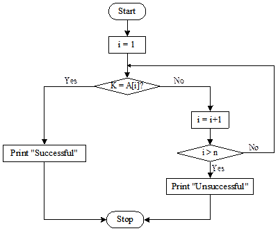
Fig. 13.2 Flowchart of the algorithm SearchArray.

 

Complexity analysis of the algorithm SearchArray

As we have already pointed out and also seen in the algorithm SearchArray, the basic operation is key comparison. We shall consider the number of comparisons require for three different cases.

 

Case 1: The key matches with the first element

This is the case when key is present in the array as the first element, that is, A[1]. In this case, only one comparison, namely in Step 2 will take place. Thus, T(n) the number of comparisons is

 

T(n) = 1                                                                                                                         

 

This case corresponds to the best case of this algorithm.

 

Case 2: Key does not exist

This is the case of searching when the key is not present in the array. In this case, the else part of the if-statement at Step 2 is executed for A[1], A[2], …, A[n], that is, n number of times. Hence, total number of comparisons T(n) in this case is   given by

 

                               T(n) = n                                                                                                                         

 

This is the case corresponding to the worst case of the algorithm.

 

Case 3: The key is present at any location in the array

Let   be the probability that the key is present at i-th location, for any 1 ≤ i ≤  n. To reach at i-th location, the algorithm executes (i-1) comparisons at Step 2. Hence, for a successful search at i-th place, we need (i-1) + 1 = i number of comparisons. So, expected number of comparisons is given by

   

                                                                                                                                          

 

For the simplicity, let us assume that the place of key is equally probable at every location. Therefore, we can write

 

               

 

Thus Equation 11.3a reduces to

 

                               

         =

         =                                                                                                                     

 

Hence, number of key comparisons, when the key is present at any location is

 

                                                                                                                                                 

 

This gives the average case behavior of the algorithm SearchArray.

 

From, the above calculations, we can write the time complexity in asymptotic notation as shown in Table 13.1.

 

Table 13.1 Summary of number of comparisons in the algorithm Search Array.

 

 

Linear Search with Linked List

In the foregoing discussion, we have considered linear searching when n elements are stored in contagious storage locations, such as array. Here, we shall consider another type of linear search method where elements are stored in a non-contagious storage in the form of linked list. We consider single linked list with two components of a node: DATA (to store value of an element) and LINK (to store the address to the next node), see Figure 13.3(a).

                A linked list structure and linear search method on it is illustrated in Figure 13.3(b). In Figure 13.3(b), H denotes the pointer to the header node. The linear search method begins with the node pointed to by the header node H. Starting from this node, it compare the key value stored in it. If key matches search successfully terminates, else moves to the next node. This process is repeated for subsequent nodes until a key matches end of the list is reached. In the later case, search is terminated unsuccessfully. 

    The algorithm for sequential search on a linked list is defined as SearchList below:

 

 

Fig. 13.3  Linked list and illustration of linear search with a linked list.

 

Algorithm SearchList

Input:     H is the pointer to the header node and K is the key to be searched.

Output: print a message “successful” if K is present else message “unsuccessful”.

Remark: Elements in the linked list are not necessarily stored in order.

 

Steps:

1.	ptr = H→LINK                                   // ptr is the pointer variable. Search starts from the first node
2.	flag = FALSE                                                                                                          // Status of search
3.	While (ptr NULL) && (flag = FALSE) do
4.		If (ptr→DATA = K) then
5.			flag = TRUE                                                                                       // Key is matched
6.		Else
7.			ptr→LINK                                                                                   // Go to the next node
8.		EndIf
9.	EndWhile                                                                                       // Linked list traversal is finished
10.	If (flag = TRUE) then                                                                                                     // K is found
11.		Print “Successful”
12.	Else                                                                                                                            // K is not found
13.		Print “Unsuccessful”
14.	EndIf
15.	Stop

 

Linear Search with Ordered List

So far we have discussed linear searching and its variations. In all the previous discussions, we assumed that elements are in random order. Next, we shall consider the linear search methods when elements are in ascending order.

               An algorithm for linear search method with ordered elements stored in an array A[1….n] is defined below.

 

Algorithm SearchArrayOrder

Input:     A[1….n] is an array of n elements and K is the key to be searched.

Output: A successful message and the location of the array element where K matches,

             otherwise an unsuccessful message.

Remark: All elements are arranged in ascending order and array index ranges from 1 to n.

 

Steps:

1.	i = 1                                                                                          // Begin search from the first location
2.	flag = TRUE                                                                                                            // Status of search
3.	While (flag ≠ FALSE) && (K  A[i]) do                                 // Don’t proceed further if K < A[i]
4.		If (K = A[i]) then                                                                                             // K is matched
5.			flag = FALSE                                                                                   // Search is over
6.			Print “Successful at”    i
7.		Else                                                                                 // Key may be in the range of search
8.			i = i + 1                                                                                // Go to the next element
			If (i > n) then                           // Check if the next element is beyond the boundary
				Break                                                                                // Quit the program
			EndIf
9.		EndIf
10.	EndWhile
11.	If (flag  = TRUE) then                                                                                          // Search is failed
12.		Print “Unsuccessful”
13.	EndIf
14.	Stop

 

The algorithm SearchArrayOrder is self-explanatory.

 

Analysis of the algorithm SearchArrayOrder

The run time behaviors of both the algorithms SearchArray and SearchArrayOrder are same so far the best case is concerned. That is, if the key is present at the first location in the array A. In case of successful search when the item of search is between 1 and n (both are inclusive) and if all keys are equally likely then the algorithm SearchArrayOrder takes essentially the same average time as the algorithm SearchArray. However, for unsuccessful search, which gives the worst case behavior of the algorithm SearchArray, the SearchArrayOrder has the same time complexity as the average case behavior. This is indeed a significant observation!

 

A summary of the above analysis is shown in Table 13.2 for ready reference.

 

 

Table 13.2 Summary of number of comparisons in the algorithm SearchArrayOrder.

 

Note: Cases mentioned in Table 13.2 are same as in the case of analysis for SearchArray algorithm.

 

Binary Search

The linear search methods discussed so far is treated as the simplest search method and works fine if the lists are small. If the lists are very large then they lead to inefficient search methods. For example, if you want to find your name in a list of names of registered students, then it is not bad to search the list from top to bottom (or bottom to top). In contrast, suppose you want to search the word “symbiosis” in your dictionary. You apply linear search starting from first page; of course, you can afford this if you want to pass your time! But, if you are in a hurry, then your intuition is to probe a page approximately at the middle of the dictionary. If you are lucky at that moment you can find the meaning there; otherwise try again in the first half or second half depending on your sense of lexicographical ordering, and repeat the same process on a half. This intuition becomes a policy of an efficient search algorithm called the binary search. It may be noted that binary search is applicable only when the list is in sorted order, like a dictionary is in lexicographic order. The mechanism of binary searching is explained below.

Let us consider an array A with all elements arranged in ascending order. Let l and u are the lower and upper indexes of the array A, respectively. We want to search an item K in it. To do this, we calculate a middle index with the values of l and u. let it be mid. Then we compare if K = A[mid] or not. If it is true then the search is done. Otherwise, the search is to be repeated on left half or right half depending on the inequalities K < A[mid] or K > A[mid], respectively. The approach of binary search technique is illustrated in Figure 11.6. It can be seen that each time value of either l or u is adjusted according to the value of K and value at the middle mid. In case of l = u and K ≠ A[mid], the search terminates unsuccessfully.

    

Fig. 13.4  Principle of binary search method.

The above concept of binary search method is presented in the form of algorithm the BinarySearch as stated below.

 

Algorithm BinarySearch

Input:     An array A[1…n] of n elements and K is the item of search.

Output: If K is present in the array A then print a successful message and return the index where it

             is found else print an unsuccessful message and return -1.

Remark: All element in the array A is stored in ascending order.

 

Steps:

1.	l =1, u = n                                                                        // Initialization of lower and upper indexes
2.	flag = FALSE                                                                             // Status of the search, initially false
3.	While(flag ≠ TRUE) and (l ≤ u) do
4.		// Calculate the index at middle
5.		If (K = A[mid]) then                                                     // K matches and search is successful
6.			Print “Successful”
7.			flag = TRUE                                                             // Status of the search is now true
8.			Return(mid)
9.		EndIf
10.		If (K < A[mid]) then                                                // Let us check for possibility in left part
11.			u  = mid-1                                                 // This is the rightmost index of the left-half
12.		Else                                                       // K > A[mid] and chaeck the possibility at right part
13.			l = mid+1                                                 // This is the leftmost index of the right-half
14.		EndIf
15.	EndWhile
16.	If (flag = FALSE) then                                                                                           // Search is failed
17.		Print “unsuccessful”
18.		Return(-1)
19.	EndIf
20.	Stop

 

 

Illustration of the algorithm BinarySearch

Let us trace the algorithm with an example. Consider an array of eight elements (see Figure 13.5). Suppose, we want to search the list for K = 75. Algorithm starts with l = 1, u = 8 (Figure 13.5(a)). The control variable flag is set as FALSE. Figure 13.5(b) show the first iteration. In this iteration, we see the value of mid = (1+8)/2 = 4. Since A[4] = 45, else part of the If-statement (Step13) is executed resulting l = 4+1 = 5 (see Figure 11.7(b )). Next, iteration 2 begins with l = 5 and u = 8 (it is the right-half of the list) and according to Step 4, mid = (5+8)/2 = 6 is calculated. Since, A[6] = 75 (see Figure 13.5(c)) the if-statement at Step 5 is executed. It prints “Successful” message, reset flag = TRUE and Return the location of K as 6 (Step 7-9) and algorithm terminates. In this illustration, we have traced the algorithm for a successful search.

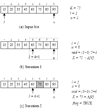
Fig. 13.5  Illustration of BinarySearch in case of successful search.

 

Now, let us consider the case of unsuccessful search. Suppose, we want to find K = 55. This is illustrated in Figure 13.6. Iteration 1 (see Figure 11.8(b)) begins with l = 1, u = 8 and according to Step 4 mid = (1+8)/2 = 4. Since A[4] = 45 and 55 > A[4], else part (at Step 13) of the if-then-else statement (at Step 10-14) is executed resulting in  l = 5 and u = 8. This is followed by the iteration 2, which is shown in Figure 11.8(c). Iteration 2 begins with the right-half of the list and as per Step 4, mid = (5+8)/2 = 6. Since, A[mid] = 75 > 55, Step 11 is executed, which results in  l =5 and u = 5. This leads to third iteration on the left part of the just concluded list. In iteration 3 (see Figure 11.8(d)), mid is calculated as mid = (5+5)/2 = 5 and Step 11 is executed giving u = 4. The iteration 4 does not roll as l = 5 and u = 4 and violating the loop condition, namely (l < u). On termination of the While-loop (Step 3-15), control goes to Step 16. Consequently  flag = FALSE, if-statement (Step 16) is executed printing the message “Unsuccessful” and returning -1; finally algorithm terminates.

 

Fig. 13.6 Continued.

 

Fig. 13.6  Illustration of BinarySearch in case of unsuccessful search.

 

Students are advised to trace the algorithm BinarySearch for K = 15, 65 and 95.  

 

Fibonacci Search

Binary search algorithm we have discussed is known to be a high speed searching method over a list of elements sorted in an order. However, binary search algorithm requires a division operation in each iteration and since division operation is a computationally expensive operation, this may steal its show. In other words, so far time of computation is concerned, it is possible to improve the speed if we can avoid this division operations. David E. Ferguson (CACM 3 (1960), 648-657) proposed a solution addressing this problem. He proposed a decision tree similar to Fibonacci tree and follows a searching method same as binary search but according to this Fibonacci tree.

      We first explain the construction of Fibonacci tree to understand the method in the Fibonacci search. We know that n-th Fibonacci number in a binary Fibonacci series is given by

 

                      with  and

 

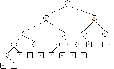
If we expand the n-th Fibonacci number into the form of a recurrence tree, it results in a binary tree and we can term this as Fibonacci tree of order n. In a Fibonacci tree, a node corresponds to F_i, the i-th Fibonacci number, its left sub tree is F_i-1 and right sub tree is F_i-2. The F_i-1 and F_i-2 are further expanded until F₁ and F₀.  A Fibonacci tree of order 6 is shown in Figure 13.7(a). The same tree can be relabeled by placing the values of F_i’s instead of F_i and is shown in Figure 13.7(b).

 

We can follow the two rules mentioned below to obtain the Fibonacci search tree of order n from a Fibonacci tree of order n.

 

Rule 1: For all leaf nodes corresponding to F₁ and F₀, we denote them as external nodes and redraw them as squares, and value of each external node is set to zero. This is shown in Figure 13.7(b).

 

Rule 2:  For all nodes corresponding to F_i (), each of them as a Fibonacci search tree of order i such that

• the root is F_i
• the left sub tree is a Fibonacci search tree of order i-1,
• the right sub tree is a Fibonacci search tree of order i-2 with all numbers increased by F_i.

 

Note: It can be noted that the Fibonacci search tree is defined recursively.

 

Following the definition of Fibonacci search tree as mentioned above, we can readily obtain a Fibonacci search tree of order n from a Fibonacci tree of order n.  For example, the Fibonacci tree of order 6 (in Figure 13.7 (b)) is converted to the Fibonacci search tree of order 6 is shown in Figure 13.7(c).

 

In any Fibonacci search tree of order n, following important observation may be noted.

 

1.      (a)  Number of internal nodes = F_n+1-1

         (b)  Number of external nodes = F_n+1

 

2.   For each internal node, if both children are internal nodes then the difference of values between a parent and any child is same and this amount is a Fibonacci value (it is the Fibonacci value for right child according to the Fibonacci tree).

 

3.   If elements are stored in an array A[1…] and arranged in ascending order, size of the array being  then the searching for a key K the location of probes is decided by traversing from root node to an internal node whose value is K, provided that the search is successful. On the other hand, if the search is unsuccessful, the probes are decided by tracing a path from root node to an external node such that,  where  denotes the elements at i-th location in the array A.

 

All these observations can be verified from the Fibonacci search tree of order 6 shown in Figure 13.7(c). 

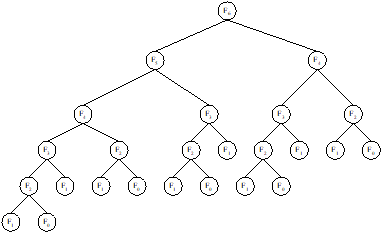
(a)   A Fibonacci tree of order 6

 

 

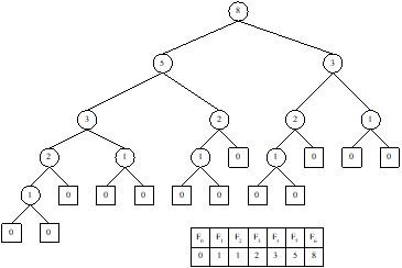
(b)   Rule 1 is applied to the Fibonacci tree of order 6

 

 

(c)    Rule 2 is applied to intermediate Fibonacci tree in Fig. 13.7 (b)

 

Fig. 13.7 Creating Fibonacci search tree of order 6.

 

The following algorithm makes a precise description for the Fibonacci search method.

 

Algorithm FibonacciSearch

Input: An array A of size n and K is the element to be searched.

Output: If K is present A then print a successful message and return the index where it is found,

             else print an unsuccessful message and return -1.

Remarks: All elements are stored in sorted order. Number of elements n is related to a perfect Fibonacci number , such that, = n+1.

Steps:

	/* Initialization */
1.	i = Fk                                                                                                               // Start at Fk-th location
2.	p = Fk-1, q = Fk-2                                            // Pointers to the left and right sub trees of the node  Fk
3.	If (K<Ki) then                                                   // Compare the key K with the value at i-th location
4.		If (q = 0) then
5.			Print “Unsuccessful”
6.			Return()                                                                                               // Serach is over
7.		Else
8.			i = i-q, pold = p, p = q, q = pold -q                                                    // Go to left sub tree
9.			Go to Step 3
10.		EndIf
11.	EndIf
12.	If (K>Ki) then
13.		If (p = 1) then
14.			Print “Unsuccessful”
15.			Return()                                                            // Search is unsuccessfully terminated
16.		Else
17.			i = i+q, p = p+q, q = q-p                                                              // Go to right sub tree
18.			Go to Step 3
19.		EndIf
20.	EndIf
21.	If (K = Ki) then
22.		Print “Successful at i-th location”
23.	EndIf
24.	Stop

 

 

Illustration of the algorithm FibonacciSearch

The Fibonacci search algorithm can be easily traced with an example, which is shown in Figure 13.8. Here, A contains 12 elements and F_k+1=12+1=13. Suppose we want to search for K = 25. Different steps are shown is Fig.13.8.

Students are advised to test the algorithm for the same input list but with (1) K = 55, (2) K =10 and (3) K = 100.

 

 

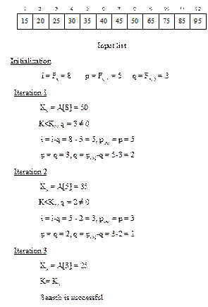
Fig. 13.8 Illustration of Fibonacci search.

 

Analysis of the algorithm FibonacciSearch

The complexity analysis of the Fibonacci search algorithm is left as an exercise to the students. The following observations regarding the time complexity to search an element from a list of n order elements can be proved with rigorous mathematical calculations.  

 

Best case

Successful search:    T(n) = 1

Unsuccessful search:  T(n) = k-1

 

Worst case 

Successful search:  

Unsuccessful search: 

 

Average case

Successful search: 

Unsuccessful search:  

 

Here, = Golden ratio = and hence . k = order of the Fibonacci search tree with n elements, that is,  F_k+1= n+1.

 

Interpolation Search

Both the binary search and Fibonacci search methods probe at around the center of the region of search. It would be better if the locations probed are not at the center rather decided by the key element itself. For example, when searching for a word in dictionary, we intuitively do not start at half initially. We start where it might be and then a large or small chunk apart depending on the currently probed and the probable location of the key. This eventually needs lesser number of probes and hence possibly an improved search method. Based on this observation, W. W. Peterson (IBM Journal of Research and Development, Vol.1, Page 131-132, 1957) suggested a search method called the interpolation search. The interpolation search calculates the next probe location using the following interpolation formula (hence, the name).

 

                                                                                    (11.14)

 

Where, K is the element to be searched within the range of elements K_l (lower end) and K_u (higher end). u and l are the upper and lower indexes of the search boundaries. In other words, if K lies between K_l and K_u, then the next probe will be at loc according to Equation 11.14. Interpolation search works only on numerical elements arranged in sorted order with uniform distribution (that is, the interval between any two successive elements are roughly a constant). The interpolation search is described using pseudo code given below.

 

Algorithm InterpolationSearch

Input:   An array A[1…n] of n elements and K is the item of search.

Output: If K is found in the array A then print a successful message and return the index where it is found else print an unsuccessful message and return -1.

Remark: The array A is sorted in ascending order.

 

Steps:

1.	l = 1, u = n                                                                                     // Initialization: Range of searching
2.	flag = FALSE                                                                                         // Hold the status of searching
3.	While (flag = FALSE) do
4.
5.		If (then                                                        // If loc is within the range of the list
6.			Case:  K < A[loc]
7.				u = loc -1
8.			Case:  K = A[loc]
9.				flag = TRUE
10.			Case:  K > A[loc]
11.				l = loc +1
12.		Else
13.			Exit()
14.		EndIf
15.	EndWhile
16.	If (flag) then
17.		Print “Successful at” loc
18.	Else
19.		Print “Unsuccessful”
20.	EndIf
21.	Stop

 

Students are advised to verify the working of the algorithm InterpolatioSearch  with the sample as used in the discussion of the algorithm FibonacciSearch.

 

Analysis of the algorithm InterpolationSearch

W. W. Peterson just formulated the interpolation search technique [1957] and its complexity were analyzed long back [in 1976] by A. C. Yao and F. F. Yao [JACM, Vol.23, Page 566-571, 1976]. Here, to make the discussion simple, we avoid the Yao-Yao calculation of time complexities.

        It is evident that the interpolation search is superior to binary search because in the binary search, in any step it reduces the region of search from n to n/2 whereas, the interpolation search reduces the same from n to. Further calculation reveals that interpolation search takes about  number of steps, on the average compared to  number of steps, on the average in the binary search.  Interpolation search proves its worst, in particular when the size of list is enormous large, like n = 2¹⁶ = 65,356 or so.

 

Summary of Linear Search Algorithms

In this section, we have discussed few important search algorithms for searching over a list of elements stored in an array or linked list. The asymptotic time complexities of all these algorithms are listed in Table.11.1.

 

Table 13.1 Comparison of linear searching methods.

Searching method	Case	Time complexity in
		Best case	Worst case	Average case
Linear search with array	Successful	1	n
	Unsuccessful	n	n	n
Linear search with list	Successful	1	n
	Unsuccessful	n		n
Binary search	Successful	1
	Unsuccessful
Fibonacci search*	Successful	1
	Unsuccessful	k-1
Interpolation search	Successful	1
	Unsuccessful

^* k is such that F_k =Key, Fk is the k-th Fibonacci number. .

 

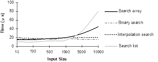
The performance curves of all search algorithms are drawn as shown in Figure13.9.

 

From the discussion of four searching algorithm in this category and from Table 13.1 and Fig.13.9, we can conclude the following.

1. Sequential search methods (both on ordered and unordered lists) are easy to write and efficient for smaller lists, but work inefficiently when the size of list is too large.
2. So far the average case complexity is concerned, interpolation search works better than any algorithm in this category but it is only applicable for numeric keys.
3. Fibonacci search is comparable to the binary search for certain values of n. For large n, Fibonacci search appears slower than the binary search algorithm. This is because, in Fibonacci search time of iteration is less but if number of iteration increases its ceases the overall impact.
4.  Binary search algorithm in fact considering overall things and treated as the best searching algorithm to search a linear list.

 

Note: It can be noted that binary search requires a sorted list; so if the list is not sorted then even with a fastest sorting method of O(nlog₂n), searching including the time of binary search needs O(nlog₂n) + (log₂n) . In contrast to sequential search, which does not require the list to be sorted, and on the average, it has the time complexity O(n). In a nutshell, binary search is preferable when it is required to search several times once the list is made. Here, one sorting operation is followed by many searching operations. On the other hand, when a list is under subject to modification (like insertion, deletion etc.) the sequential search is preferable.

 

 

 

 

(a) Successful search

 

 

 

(b) Unsuccessful search

 

Fig. 13.9  Performance of different linear search algorithms.

 

 

 

 

 

 

 

NONLINEAR SEARCH TECHNIQUES

In the last section of this chapter, we have learned searching methods when elements are stored in a linear data structure such as array or linked list. We also know that insertion/deletion operation with this data structure involves a large number of data movements and hence time consuming. As a consequence, this type of storage structure is not preferable in applications where frequent insertion or deletion operations are involved. In order to avoid this problem, programmers prefer to use nonlinear data structures such as tree, graph, etc. In these type of data structures insertion and deletion operations are faster compared to the linear data structure. Apart from this, it is also observed that nonlinear data structures are preferable for faster search operation. In this section, we shall study important searching methods those deal with nonlinear data structures. All nonlinear searching methods discussed in this chapter are classified as shown Figure 13.10. All nonlinear search techniques can be classified into two categories: tree searching and graph searching. All tree-based searching methods are involved with data, which are stored in binary trees.  In our tree search we consider searching a binary tree and its variations. On the other hand, graph-based searching methods deal with data, which are stored in a graph structure. A graph structure is same as the tree structure except that the former is acyclic. In the following subsections we cover all the searching methods shown in Figure 13.10.

 

 

 

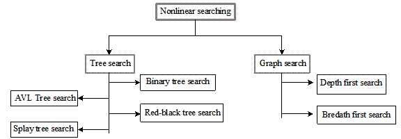
Fig. 13.10  Nonlinear searching techniques.

 

Binary Tree Searching

We assume   the prerequisite of understanding binary tree, in particular, the storage representation of a binary tree. In an abstraction, we consider a binary tree simply in the form of a tree, where each node has at most two children. Each node stores an element. Number of nodes in a binary tree is same as the number of elements from which a given key element to be searched. A binary tree with 10 elements is shown in Figure 13.11. Note that all nodes are unique, that is, no two nodes store same numbers.

 

 

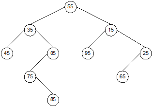
Fig. 13.11 A binary tree storing 10 elements.

 

Given a binary tree, our problem is to search whether an element present in it or not. A simple method to do this is to traverse every node in it and check whether the given element present in any node or not. There are three ways that such a traversal can be done: preorder, inorder and postorder traversals. All these three binary tree traversals are discussed in Chapter 7, Section 7.4.3. Here, we present the preorder tree traversals only from the searching perspective. Other tree traversals can be defined accordingly.  Searching an element stored in a binary tree following preorder tree traversal is presented in the form of algorithm BinaryTreeSearch.

 

Algorithm BinaryTreeSearch

Input:     A binary tree with PTR  as the pointer to a node and K is the element under search.

Output: Returns 1 if K is available, otherwise returns NULL.

Remark: Algorithm follows preorder traversal and is defined recursively.

            

Steps:

1.	ptr = PTR                                                                  // Start from the current node of the binary tree
2.	If (ptr  NULL)  then
3.		If (ptr→DATA = K) then                               // Visit: Check the element in the current node
4.			Return (1)                                                                        // Return the status of search
5.		Else
6.			BinaryTreeSearch (ptr→LC)                    // Then search the left sub tree in preorder
7.			BinaryTreeSearch (ptr→RC)                 // Then search the right sub tree in preorder
8.		EndIf
9.	EndIf
10.	Stop

 

 

 

 

Illustration of the algorithm BinaryTreeSearch

Suppose ROOT is the pointer to the root node of a binary tree. To search the binary tree, we call the algorithm BinaryTreeSearch with ROOT as an argument. The algorithm BinaryTreeSearch follows preorder traversal and how the searching of 95 will take is explained in Figure 13.12. The order in which different nodes are visited is labeled as 1, 2, …, 8. It is observed that at 8-th visit we find the match. It can be noted that unlike the preorder tree traversal the algorithm BinaryTreeSearch does not visit all nodes and terminates as soon as it finds the match by retuning 1 (Step 4). In case of an unsuccessful search however, it traverses every node and finally returns with NULL.

 

 

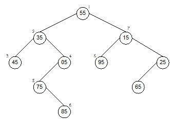
Fig. 13.12  Illustration of BinaryTreeSearch algorithm.

 

 

Analysis of the algorithm BinaryTreeSearch

Let us assume that the basic operation in the algorithm BinaryTreeSearch is the key comparisons. The number of comparisons required in this method, in fact, depends on the structure of tree. For example, let us consider three binary trees as shown in Figure 13.13. Three skewed (also called degenerate) binary trees are shown in Figure 13.13(a). In case of searching 95 in the trees we need only 1 key comparison, whereas for the key 55 it requires 10 key comparisons (see Figure 13.13(a)). Now, consider another extreme of the binary tree shown in Figure 13.13(b). This is a complete binary tree and all levels contain maximum number of nodes except possibly the last level. How many key comparisons we need to search any element in it? Let us calculate this for a binary tree with n nodes. Let us denote p_i as the probability that searching an element requires i number of key comparisons. Since, number of key comparisons varies from 1 to n, we can find average number of key comparisons as

 

                                                                                                                      

 

Let us assume that an element is equally probable in any nodes. With this assumption we have

 

                                                                                                                                  

              

From Equation 11.15 and Equation 11.16, we have on the average, number of key comparisons

 

=  =                                                                                      

 

Therefore, with reference to the binary tree shown in Figure 13.13(b), we say that the number of key comparisons, on the average  5. In fact, this result (Equation 13.13(b) is true for any binary tree structures.

 

We now summarize the above results. Let T(n) denotes the number of key comparisons required in a binary tree with n number of nodes in it.

 

Successful search

 

Minimum number of key comparisons

The minimum number of key comparisons required is 

 

T(n) = 1                                                                                                                       

 

Maximum number of key comparisons

The maximum number of key comparisons required is 

 

T(n) = n                                                                                                                     

 

Average number of key comparisons

On the average, number of key comparisons required is

 

                                                                                                            

 

All these results are tabulated with the big-oh asymptotic notation in Table 13.2.

 

 

Table 13.2 Summary of number of comparisons in the algorithm BinaryTreeSearch.

 

 

 

 

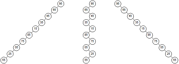
(a)    Three skewed binary trees with same set of data

 

 

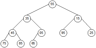
(b)    A complete binary tree

 

Fig. 13.13  Analysis of BinaryTreeSearch algorithm.

 

 

Binary Search Tree Searching

Binary search tree (also called binary sorted tree) is a special tree, where node satisfies the following property.

         If n is any node in the binary search tree then the value of n is greater than any value in the left sub tree and less than any value in the right sub tree (see Figure 13.14(a)). Note that in a binary search tree two nodes with equal values are not allowed (this never arise for a list of key elements, which are necessarily to be unique).

        Suppose, all elements are stored in the form of a binary search tree and K be the element to be searched. The searching operation begins at the root node. If the elements stored at the root node then search is successful and search stops here else if K is less than or greater than the element at the root node then we repeat the same procedure but at the left or right sub tree, depending on whether K is less than or greater than the element at the root node.

The above method can be precisely expressed with an iterative definition as stated below. We assume that binary search tree is represented with linked structure (Figure 13.14(b)). ROOT is the pointer to the root node, and K the item to be searched.

 

// Iterative definition of a binary search tree searching //

 

Algorithm BinarySearchTreeSearch

Input:    ROOT is the pointer to the root node and K is the item to be searched.

Output: Print “Successful” or “Unsuccessful” message if K is found or not, respectively.

 

 Steps:

 

 

The same procedure of searching a binary search tree is given below but with the recursive definition.

// Recursive definition of binary search tree searching//

 

Algorithm BinarySearchTreeSearch

Input:    ROOT is the pointer to the root node and K is the item to be searched.

Output: Print “Successful” or “Unsuccessful” message if the key K is found or not, respectively.

Steps :

1.	If (ptr = NULL) then                            // Termination condition
2.		Print “Unsuccessful”
3.		Return
4.	EndIf
5.	If (K = ptr→DATA) then
6.		Print “Successful”
7.		Return
8.	Else
9.		If (K < ptr.DATA) then
10.			BinarySearchTreeSearch(ptr→LCHILD, K)          // Repeat at the left sub tree
11.		Else                                                                                                         // K > pt→DATA
12.			BinarySearchTreeSearch(ptr→RCHILD, K)        // Repeat at the right sub tree
13.		EndIf
14.	EndIf
15.	Stop

 

Note that the routine as defined recursively should be called from a main routine with arguments ROOT and K. The algorithms are straight forward and easy to understand. Students are advised to exercise the algorithms with the binary search tree shown in Figure 13.14(c) for the elements 54 and 95.

 

 

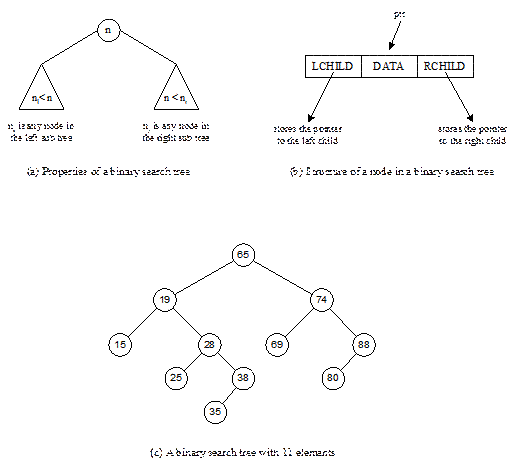
Fig. 13.14 Binary search tree revisited.

 

 

 

 

 

 

Analysis of the algorithm BinarySearchTreeSearch

Consider a binary search tree with n key elements. To analyze the time complexity of search operation in a binary search tree, we consider an extended binary tree. For example, an extended binary search tree where square vertices are drawn replacing all the NULL links is shown in Figure 13.15. With an extended binary search tree, we can say that a successful search always terminates at an internal node (drawn as circle) and an unsuccessful search always terminates at a leaf node.

 

 

Fig. 13.15 A binary search tree and its extended binary search tree version.

 

It is obvious that searching time depends on two things: the position of the key in the binary search tree and height of the binary search tree. For example, if the key is at the root then we are fortunate to find that at the earliest. On the other hand, if the key is at the last level then we are to visit all keys in the path starting from the root to that node at the last level. Further, for a same set of keys binary search tree is not unique rather it depends on the arrangement of the keys. Given a binary search tree therefore, the search time depends on the structure of the tree as well.

Following points are pertinent and useful in order to analyze the complexity of the algorithm.

 

·         We assume that the comparison of keys is the basic operation in the algorithm BinarySearchTreeSearch (both iterative and recursive definitions). It may be noted that as we consider key comparisons, so condition checks (termination in recursive or while loop in iteration etc.) will not be taken into consideration.

·         While visiting a node, for every unmatch it requires two comparisons. For every match (which occurs at an internal node) it requires one comparison. For every unsuccessful match (which occurs at an external node) it requires one comparison.

·         Successful search terminates at an internal node. If successful search occurs after visit to m number of nodes, then the total number of comparisons required is 2(m-1)+1=2m-1. Here, first (m-1) nodes are visited corresponding to unmatch and the last m-th node is visited to a match.

·         Unsuccessful search terminates at an external node. If an external node visited after the visit of m internal nodes, then number of comparisons required is 2×m+1=2m+1.

 

In order to analyze the algorithm BinarySearchTreeSearch, we identify three cases of binary search tree structure: with maximum height, minimum height and an arbitrary height in between minimum and maximum. These three cases are corresponding to the three different cases in the complexity analysis of binary search tree searching time. Suppose, there is a list of n key elements and hence the binary search tree with n number of internal nodes. The three cases of the BinarySearchTreeSearch algorithm are analyzed below.

                                 

Case 1: Binary search tree with maximum height

A binary search tree with maximum height occurs if it is a skewed binary search tree. Some skewed binary search trees are shown in Fig. 13.16 (a). We know that the maximum height of a skewed binary search tree with n number of nodes is given by:

                                

                                                              h_max = n                                                                                       

Successful search:

Let us consider the case of successful search. Minimum number of comparisons occurs when the key is matched at the first node (see Fig. 13.16(b)). Denoting S(n) as the number of comparisons in case of a successful search in a binary search tree with n number of nodes, we have the minimum number of comparisons as

 

                                                  S_min(n) = 1                                                                                               

 

 

 

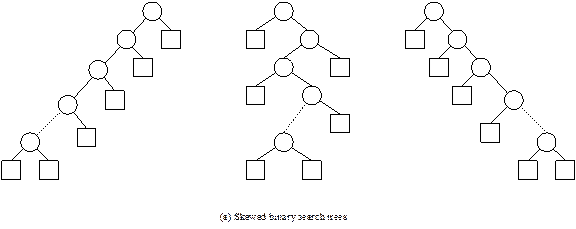
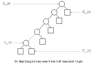
Fig. 13.16 Continued.

 

Fig. 13.16 Different binary search tree structures.

 

 

Now, maximum number of comparisons occurs when key matches the internal nodes at the deepest level. Hence, the maximum number of comparisons S_max(n) is given by

 

                                      S_max(n) = 2(h_max-1)+1

 

                                                  = 2n-1                       Since, h_max = n  [see Equation 11.20]

 

Thus,

                                     S_max(n)  = 2n-1                                                                                                    

 

Unsuccessful search:

Minimum number of comparisons occurs when the search ends at the external node at level 1 (see Fig. 11.19(b)). Let U(n) be the number of comparisons when the search is unsuccessful in a binary search tree with n number of nodes. Thus, minimum number of comparisons in case of unsuccessful search is

 

                            U_min(n) = 2 + 1 = 3                                                                                                      

 

Maximum number of comparisons occurs when the search stops at an external node at the last level. The external node in this case at the level (n+1)-th level, that is, in a path with n number of internal nodes followed by the external node. Hence, the number of comparisons is given by

                        

                             U_max(n) = 2×n + 1                                                                                                       

 

 

Case 2: Binary search tree with minimum height

The minimum height of a binary search tree (see Fig. 13.16(c) is given by

 

                        h_min =                                                                                                                     

 

With this information in mind we can analyze the number of comparisons in case of search is successful and unsuccessful as below.

 

Successful search:

Following the same argument as in Case 1, minimum number of comparisons is

 

                                     S_min(n) = 1                                                                                                         

 

And maximum number of comparison is

 

                                  S_max(n) = 2(h_min-1)+1

                                         

                                             = 2-1                                                                                   

 

Unsuccessful search:

Here, the minimum number of comparisons occurs at the last level, which is h_min +1 (see Fig. 13.16(c)). Hence, the number of comparisons is

 

                               U_min(n) = 2h_min+1        

 

                                           = 2  +1                                                                                    

 

Maximum number of comparisons also occurs at an external node, which is at the last level. Thus the number of comparisons is given by

 

        U_max(n) = 2h_max+1

                     = 2 +1                                                                               

 

 

Case 3:  Binary search tree with an arbitrary height

This is the case which is more realistic, in the sense that keys are usually appear in a random order and thus resulting in a binary search tree of arbitrary height (see Fig. 13.16 (d)) in between n (maximum) and   (minimum).

We know that the structure of a binary search tree is decided by the initial ordering of the input list (that is, the order in which elements in the list are inserted into a binary search tree starting from an empty binary search tree). Let us assume that each of the n! possible orderings of the n key elements are equally likely in building the binary search tree. We denote S(n) the number of comparison done in average successful search and U(n) the number of comparisons in the average unsuccessful search in a binary search tree of n nodes. One interesting fact is that the number of comparisons needed to find a key is exactly one more than the number of comparisons that are required to insert that key into the tree. We therefore have a relationship

 

                                                                        

 

Let I and E are the internal and external path lengths of an extended binary search tree  with n number of nodes, respectively. We can establish a relation between S(n), I and U(n)  and  E as discussed below.

Since the algorithm BinarySearchTreeSearch does two comparisons for each internal node except for the node that matches the key, and note that the number of these internal nodes traversed is one more than the number of edges. We therefore obtain the average number of comparisons for a successful search with n number of nodes in a binary search tree is given by

 

                                                                                                    

 

Here,   denotes the average path length of internal nodes. The subtraction of 1 corresponds to the fact that one fewer comparison is required when the key matches the target node. Thus,

 

                                                                                                             

 

For an unsuccessful search, we know that it leads to any one of the leaf node in the extended binary search tree. Since, there are (n+1) leaf nodes and all are equally likely, the average number of comparisons for an unsuccessful search is given by

 

                                                                                                          

 

Further, from Lemma 8.6, we know that

 

E = I+2n                                                                                                                      

 

Thus, we get

 

                                                                                                          

 

And from equation (11.32), we get

 

                                                                                                      

 

Combining Equation 11.33, 11.34 and 11.35, we get

 

                                                                                             

 

Finally, we get

 

                                                           

 

The above equation  is a recurrence relation and can be solved as follows.

 

 Writing (n-1) for n, we get

 

                                                  

 

Thus,

 

  =  4 + U(n-1)

 

or

 

                                                     

 

Expanding this recurrence relation, we get

 

                   Assuming U(0) = 0

 

       

where is called the n-th Harmonic number.

 

Substituting the value of U(n) in Equation 11.35, we get

 

            =                                       [After simplification]

Since, the n-th harmonic number can approximately be written as, and for large values of n, taking we get two important results mentioned below.

 

                                                                                                     

 

                                                                                             

 

Above results are summarized in Table 13.3.

 

Table 13.3 Summary of number of comparisons in the algorithm BinarySearchTreeSearch.

	Successful search		Unsuccessful search		Remark
	Minimum number of comparisons	Maximum number of comparisons	Minimum number of comparisons	Maximum number of comparisons
Case 1	1				Best
Case 2	1	2n-1	3	2n+1	Worst
Case 3	1				Average